ACT 1. Not much data...

"Get me more data, will you?" shouted Jay, the experimenter sitting at the computer impatiently, obviously frustrated and disoriented at the

that his associate Pixo managed to record that day from the only human subject they have had in months, a period that passed like years. "I'm afraid that's all we have for today because Polo is already walking home." Polo had been suffereing from a serious brain disorder and offerred to be the guinea pig for that day, but did not yet learn to entertain the experimenters well enoungh by sitting idle and involving in the impossible task of staring at blank walls for long durations. "Oh no! Look Pixo, you got to be more efficient than this. What do you want me to do with . Publish in Scientific American? How about our college research journal?" Jay is already walking out and his computer's classic shutdown music added a background score to the drama that just occurred.

ACT 2. Lots of data, but...

Ray is a modeler and computational data analyst who is interested in finding frequencies and varying time scales in the

(such as spike times) that he collected. So he naturally uses auto- and cross-correlation methods, and sets out on a long and laborious journey of determining the time constants. The methods produced frequencies and time constants for any given segment of the data, but when he chose to alter the bin width sligthtly, all the previous results appeared to diagree with the new results. Previous suggestions on the choice of bin width didn't seem to apply to his data. He knows he is faced with the problem of , and having tons of data did not help him.

What is the problem?

The two case scenarios described above are rampant in experimental and computational data analysis. More often than not, the data is non-stationary, and equally often the data set is too short (fewer points) for analysis. The problems are compounded by the requirement of an appropriate bin width for correlation functions, and data in multiples of an integer for other spectral analyses. There perhaps is no single silver bullet for all the problems faced while analyzing such

. But finding correlations would seem the first basic anslysis one should do. Correlation methods assume stationarity. Adding tons of data to get a "nice" correlation profile is not the correct analysis. One would wish for a method that could detect any existing correlations even in brief data sets, and could also predict the auto- or cross-correlations when the data is long engouh. All the better if bin width is taken out of the analysis because there is no thumb rule that works best for such data.

But first, what is the problem again with correlation function?

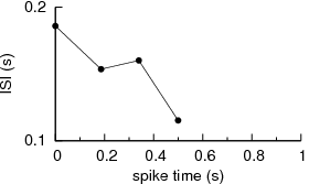
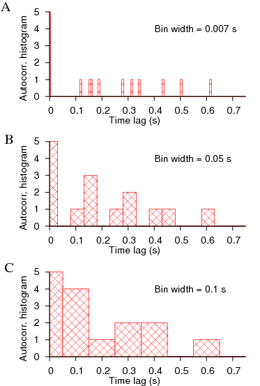
Simply put, the correlation functions assume stationarity of the data, and changes in frequency in the data or patterns of irregularity would be glossed over when lot of data points are included in the computation. One could work with brief data in an attempt to overcome the problems with non-stationarity, but one faces the problem of bin width that alters the computation giving inconsistant picture. For example, let us consider

from an experiment. These are the times at which an event occurred. When difference of successive events is taken, it gives four inter-event intervals or inter-spike intervals(ISI) as displayed in the figure below.

Now let us examine the autocorrealtion function computed for these five data points. For computing the autocorrelation, you need to use a . We show below the function computed for three different bin width sizes.

The correlation functions are computed using the binning mechanism when pairs of events are examined for a specific amount of separation, and are binned at that specific separation. As the separation (or time lag) between the trains (or between the train and its own copy) is increased, the profile of the correlation function is revealed, from which one can read off the underlying periodicity, and the time constant may be computed by integrating the absolute area under the curve.

The disadvantage of using correlation function methods for brief data is evident from the functional forms computed in the above figure. We cannot determine with certainty whether the signal represented a periodic signal, periodic signal with external noise, or totally random. The autocorrelation obtained for a bin width of 0.05 s appears to have periodicity with decaying magnitudes of the peak amplitudes. But there is no reliable method to choose this particular value of the bin width than other choices.

The problem is compounded when we seek time constant underlying the data. Determination of the time constant requires that the area under the correlation function be computed. Using different bin widths leads to different misleading time constants because there are not sufficient number of points to estimate accurately the correlation histogram with a functional curve that can be independent of bin width.

To circumvent the difficulties associated with bin widths, smoothing or filtering techniques may be employed, but again such methods do not address the case when the correlation function itself cannot be constructed in a reliable manner. They also assume stationarity of the underlying process.

What is the new method about?

After having to stare at such non-stationary data for months, it was clear to us that a new method was needed to address such data. It could do averaging, but cannot rely on including large number of data points. On closer examination of the mutual relationship between any two given spike sequences, the concept that emerged as the powerful was idea of relative time shifts between the spike trains. It is similar to that used in computing correlation functions, but not the same. Every time there is a spike event, that neuron is affecting the other neuron (against which we seek correlations) in some direct way, so that that frozen frame of relative time shifts between the spike trains must contribute to determine the mutual correlations. Assumption of a causal relationship between the spike trains is implicit in computing the correlations. Such frozen frames can be constructed by time shifting one spike sequence against the other. In each such frame, the information is contained in the relative time shifts (with respect each neuron's oscillation period at that time). This set of relative time shifts (which we call phase pairs) may live in a high dimensional space which might need separate tools to deal with. But as a first order attempt, we can look at them in a two dimensional space, and examine whether we can extract the component that is most suitable for describing correlations and deliniate it from that describing just the dissimilarity between them. The figure (a) below shows the method of constructing the phase pairs (gamma, delta) between two spike trains.

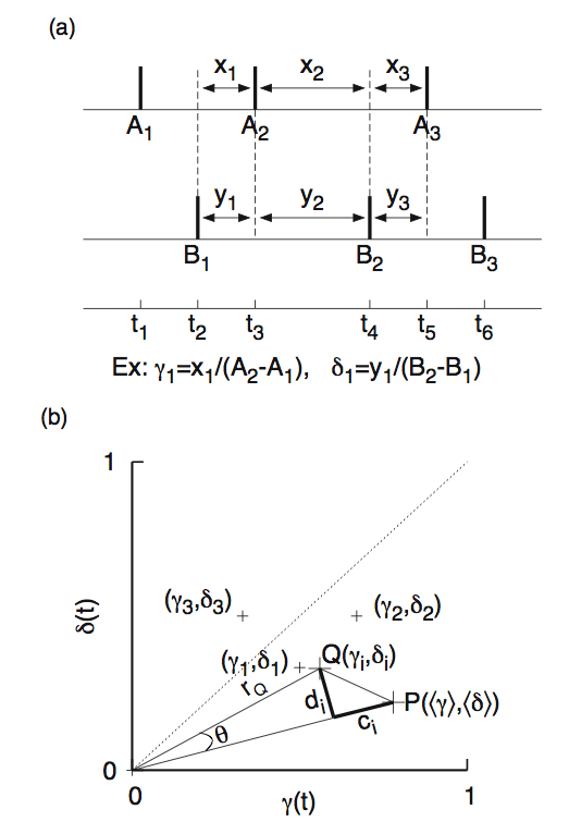
In the figure (b) above we have transformed these pairs onto a two-dimensional phase plane whose axes are normalized phases representing period of each neuron. This projection onto two dimensional plane may have cost us some valuable information that is hidden in these phase pairs, but this is the simplest transformation that helps us in identifying the component that represents the effective "drift" vs. effective "diffusion" between the spike trains. The point P represents the average point of the phase pairs, and Q is a typical point. The component c_i represents the "drift" of the point Q from the mean position P. The component d_i represents "diffusion" which we are not concerned here. An examination of each of the expressions for c_i and d_i would make this terminology more clear. Our phase function is simply quantificatiokn of these drift terms c_i. We take the avearage of the absolute values of c_i and normalize the result with the maximum value any c_i can ever attain.

A simile might help in appreciating this term better. Imagine the phase pairs as a swarm of bees around a beehive located on the branch of a tree. The drift experienced by each bee is the absolute (outward or inward) distance along the branch they find themselves with respect to the center of the beehive. The phase function is now proportional to the mean of all those drifts normalized with the maximum such value a phase pair can ever assume.

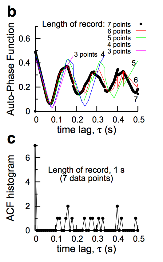
We now test this definition and compute it between a spike train and a time shifted copy of itself, i.e. an auto-phase function similar to an autocorrelation function. Our data is, of course, very short. It consists of a meager 7 spike times or less. We show the auto-phase function below in figure (b) for data points 3, 4, 5, 6, and 7, and a corresponding autocorrelation function (ACF) histogram for 7 data points in figure (c). The reults of the auto-phase function are stunning. The phase function could detect the periodicity even in 4 spike times. There is no smoothing we have employed other than the average that is already built into the definition of the phase function. On the otherhand, the autocorrelation function is not yet well formed for 7 data points; It would take some massaging of the output profile in order to clearly see the underlying periodicity.

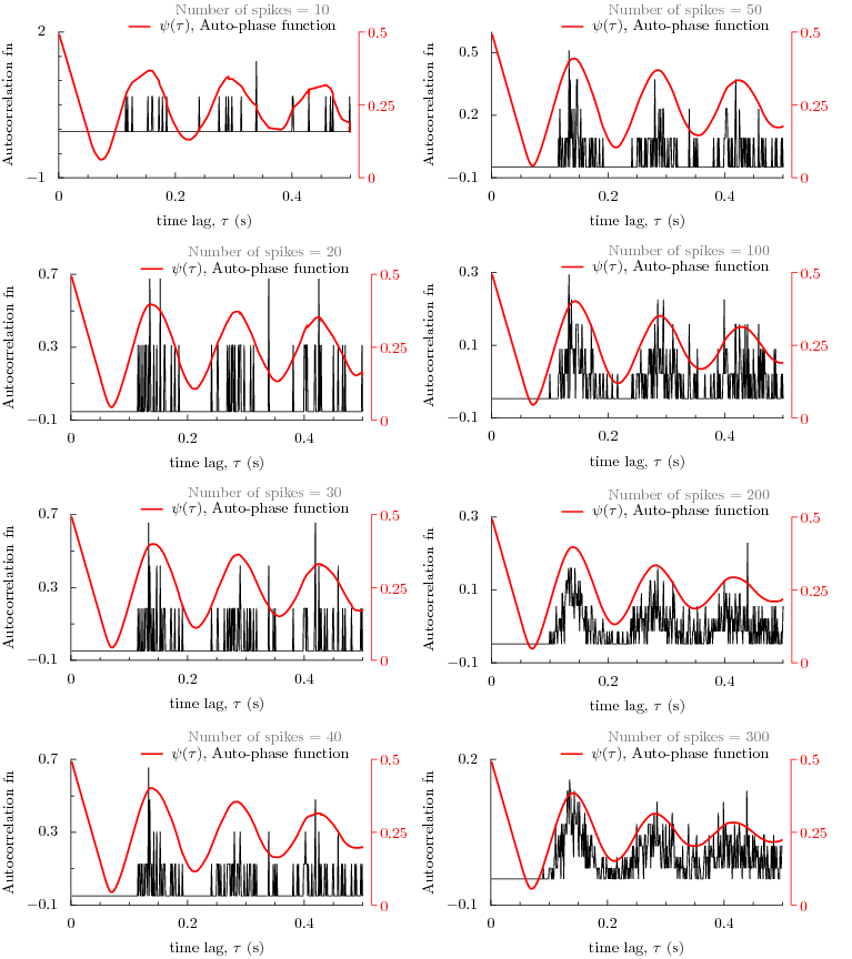
How does the phase function compare with correlation function for large number of data points?

The following figure displays a comparison between the auto-phase function and autocorrelation function for different number of data points from 10 to 300. As the number of points is increased, we see that the auto-phase function predicts the same periodicity as that of autocorrelation function.

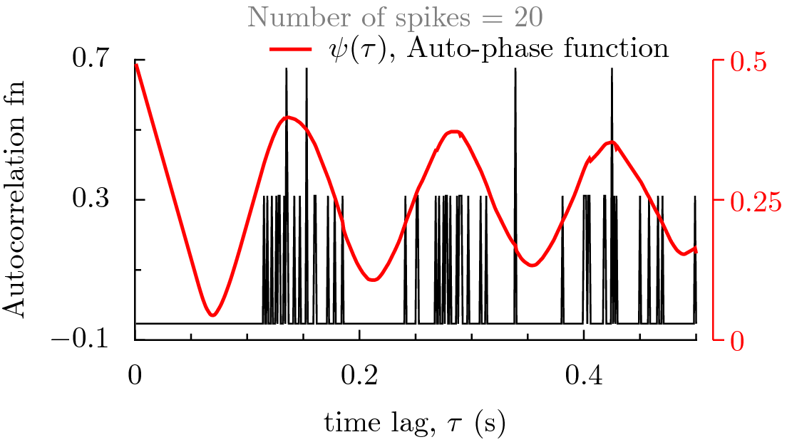
Or examine the results in the following figure by interacting with it. The data set contains 673 data points from a recording of 100 seconds of a globus pallidus neuron of rat brain slice. By choosing a number, a figure is displayed that has autocorrelation function and phase function already computed and plotted. As the number of data points is increased, we begin to see that the autophase function predicts exactly the same periodicity as the autocorrelation function.